Difference between revisions of "Word associations"
m |
|||
| (6 intermediate revisions by 3 users not shown) | |||
| Line 3: | Line 3: | ||
Giving a word as a stimulus, different persons respond with different words, e.g. “music” as stimulus can evoke “violin”, “Chopin”, “love”, “melody”, etc. Asking many persons one can observe that the frequency of particular responses (associations) is not equal, on the contrary, the response words can be ranked according to their frequency. The problem is to find the adequate ranking (<math> \rightarrow</math>) distribution. Associations are thus both ranking and diversification problems. | Giving a word as a stimulus, different persons respond with different words, e.g. “music” as stimulus can evoke “violin”, “Chopin”, “love”, “melody”, etc. Asking many persons one can observe that the frequency of particular responses (associations) is not equal, on the contrary, the response words can be ranked according to their frequency. The problem is to find the adequate ranking (<math> \rightarrow</math>) distribution. Associations are thus both ranking and diversification problems. | ||
| − | Not considering qualitative work and compilation of frequency lists having mostly the character of voluminous books, the first attempt at modelling was probably made by Horvath (1963) who used inductively the Yule distribution. Haight (1966) compared the Borel, the Yule, the logarithmic distributions with the distribution derived by him for this purpose called now Haight-zeta distribution (cf. Wimmer, Altmann 1999) but none of them could yield adequate results. Haight and Jones (1974) as well as Lánský and Radil-Weiss (1980) tried another approach but attained good results only in about 50% of cases. Dolinskij (1994, 1988) used for this purpose the Zipf-Alekseev distribution which is a generalization of Zipf distribution. Altmann (1992) has shown that the deviations from this distribution are extremely small (P ≈ 1 in almost all cases) but the foundation of this distribution was | + | Not considering qualitative work and compilation of frequency lists having mostly the character of voluminous books, the first attempt at modelling was probably made by Horvath (1963) who used inductively the Yule distribution. Haight (1966) compared the Borel, the Yule, and the logarithmic distributions with the distribution derived by him for this purpose, called now Haight-zeta distribution (cf. Wimmer, Altmann 1999), but none of them could yield adequate results. Haight and Jones (1974) as well as Lánský and Radil-Weiss (1980) tried another approach but attained good results only in about 50% of cases. Dolinskij (1994, 1988) used for this purpose the Zipf-Alekseev distribution which is a generalization of Zipf distribution. Altmann (1992) has shown that the deviations from this distribution are extremely small (P ≈ 1 in almost all cases) but the foundation of this distribution was established by Hřebíček (1995, 1996, 1997). Altmann (1992) used the usual proportionality approach with speaker-hearer balance and obtained the negative binomial distribution. |
| + | |||
'''2. Hypothesis''' | '''2. Hypothesis''' | ||
''The ranking of word associations abides by a regular ranking distribution''. | ''The ranking of word associations abides by a regular ranking distribution''. | ||
| + | |||
'''3. Derivation''' | '''3. Derivation''' | ||
| + | |||
'''3.1. The Zipf-Alekseev model''' (Hřebíček 1997: 43) | '''3.1. The Zipf-Alekseev model''' (Hřebíček 1997: 43) | ||
| Line 15: | Line 18: | ||
Hřebíček starts from two assumptions: | Hřebíček starts from two assumptions: | ||
| − | (i) The frequency of an association <math>f_x</math> at any rank x is proportional to the frequency at the first rank <math>f_1</math>. | + | (i) The frequency of an association <math>f_x</math> at any rank <math>x</math> is proportional to the frequency at the first rank <math>f_1</math>. |
| + | |||
| + | (ii) The frequency <math>f_x</math> at rank <math>x</math> is inversely proportional to the rank <math>x</math>. | ||
| − | |||
Putting this together, we obtain | Putting this together, we obtain | ||
| Line 24: | Line 28: | ||
or, in logarithmic form | or, in logarithmic form | ||
| − | <math>\ln (f_1/ | + | <math>\ln (f_1/f_x) \approx \ln x</math> |
The proportionality is given by Menzerath´s law, i.e. | The proportionality is given by Menzerath´s law, i.e. | ||
| − | (1)<math>\ln(P_1/ | + | (1) <math>\ln(P_1/P_x) = \ln(Ax^b) \ln x \quad</math> . |
| − | Solving for | + | Solving for <math>P_x</math> yields |
(2)<math> P_x = P_1 x ^{-(a+b\ln x)}\quad</math>. | (2)<math> P_x = P_1 x ^{-(a+b\ln x)}\quad</math>. | ||
| Line 36: | Line 40: | ||
Usually <math>P_1</math> is so important that one gives it a special value, i.e. one modifies the distribution obtaining | Usually <math>P_1</math> is so important that one gives it a special value, i.e. one modifies the distribution obtaining | ||
| − | (3)<math> P_x = begin{cases} \alpha, & x = 1 \\ \frac{(1-\alpha)x^{-(a+b \ln x)}}{T}, & x = 2,3,...,n \end{cases}</math>. | + | (3) <math> P_x = \begin{cases} \alpha, & x = 1 \\ \frac{(1-\alpha)x^{-(a+b \ln x)}}{T}, & x = 2,3,...,n \end{cases}</math>. |
with <math> T = \sum_{j=2}^n j^{-(a+b \ln j)}, a, b \epsilon \Re \quad, n \epsilon N, \quad 0 < \alpha < 1</math>. | with <math> T = \sum_{j=2}^n j^{-(a+b \ln j)}, a, b \epsilon \Re \quad, n \epsilon N, \quad 0 < \alpha < 1</math>. | ||
| + | |||
'''3.2. The negative binomial model''' (Altmann 1992) | '''3.2. The negative binomial model''' (Altmann 1992) | ||
| − | Assumption: The probability <math>P_x</math> at rank x is proprotional to the probability <math>P_{x-1}</math> at rank x-1, the proportionality being g(x) = (a+bx)/(cx). If ranking begins with x = 1, one solves the equation for the displaced form, i.e. | + | Assumption: The probability <math>P_x</math> at rank <math>x</math> is proprotional to the probability <math>P_{x-1}</math> at rank <math>x-1</math>, the coefficient of proportionality being <math>g(x) = (a+bx)/(cx)</math>. If ranking begins with <math>x = 1</math>, one solves the equation for the displaced form, i.e. |
| − | (4)<math> P_{x+1} = \frac{a+bx}{cx}P_x</math> | + | (4) <math> P_{x+1} = \frac{a+bx}{cx}P_x</math> |
and after reparametrization one obtains the 1-displaced negative binomial distribution | and after reparametrization one obtains the 1-displaced negative binomial distribution | ||
| − | (5)<math> P_x = {k+x-2 \choose x-1}p^k q^{x-1}, \quad x=1,2,3,...</math> | + | (5) <math> P_x = {k+x-2 \choose x-1}p^k q^{x-1}, \quad x=1,2,3,...</math> |
| + | |||
| + | where <math>a/b = k-1</math>, <math>b/c = q</math>. | ||
| − | + | '''Example''': Associations of the word “high” | |
| − | |||
Altmann (1992) used the associations of the word “high” (4th grade, male) from Palermo, Jenkins (1964) and obtained the result presented in Table 1 and Fig. 1. | Altmann (1992) used the associations of the word “high” (4th grade, male) from Palermo, Jenkins (1964) and obtained the result presented in Table 1 and Fig. 1. | ||
| − | <div align="center">[[Image: | + | <div align="center">[[Image:Tabelle11_WA.jpg]]</div> |
| Line 62: | Line 68: | ||
Both results are excellent. | Both results are excellent. | ||
| − | '''4. Authors:''' G. Altmann, J. Eom | + | |
| + | '''4. Authors:''' U. Strauss, G. Altmann, J. Eom | ||
| + | |||
'''5. References:''' | '''5. References:''' | ||
Latest revision as of 11:34, 16 June 2009
1. Problem and history
Giving a word as a stimulus, different persons respond with different words, e.g. “music” as stimulus can evoke “violin”, “Chopin”, “love”, “melody”, etc. Asking many persons one can observe that the frequency of particular responses (associations) is not equal, on the contrary, the response words can be ranked according to their frequency. The problem is to find the adequate ranking ( ) distribution. Associations are thus both ranking and diversification problems.
Not considering qualitative work and compilation of frequency lists having mostly the character of voluminous books, the first attempt at modelling was probably made by Horvath (1963) who used inductively the Yule distribution. Haight (1966) compared the Borel, the Yule, and the logarithmic distributions with the distribution derived by him for this purpose, called now Haight-zeta distribution (cf. Wimmer, Altmann 1999), but none of them could yield adequate results. Haight and Jones (1974) as well as Lánský and Radil-Weiss (1980) tried another approach but attained good results only in about 50% of cases. Dolinskij (1994, 1988) used for this purpose the Zipf-Alekseev distribution which is a generalization of Zipf distribution. Altmann (1992) has shown that the deviations from this distribution are extremely small (P ≈ 1 in almost all cases) but the foundation of this distribution was established by Hřebíček (1995, 1996, 1997). Altmann (1992) used the usual proportionality approach with speaker-hearer balance and obtained the negative binomial distribution.
2. Hypothesis
The ranking of word associations abides by a regular ranking distribution.
3. Derivation
3.1. The Zipf-Alekseev model (Hřebíček 1997: 43)
Hřebíček starts from two assumptions:
(i) The frequency of an association  at any rank
  is proportional to the frequency at the first rank
  .
.
(ii) The frequency  at rank
  is inversely proportional to the rank
  .
.
Putting this together, we obtain

or, in logarithmic form

The proportionality is given by Menzerath´s law, i.e.
(1)  .
.
Solving for  yields
(2) .
.
Usually  is so important that one gives it a special value, i.e. one modifies the distribution obtaining
(3)  .
.
with  .
.
3.2. The negative binomial model (Altmann 1992)
Assumption: The probability  at rank
  is proprotional to the probability
  at rank
  , the coefficient of proportionality being
  . If ranking begins with
  , one solves the equation for the displaced form, i.e.
(4) 
and after reparametrization one obtains the 1-displaced negative binomial distribution
(5) 
where  ,
,  .
.
Example: Associations of the word “high”
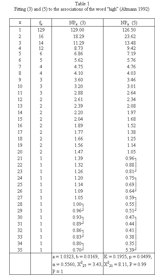
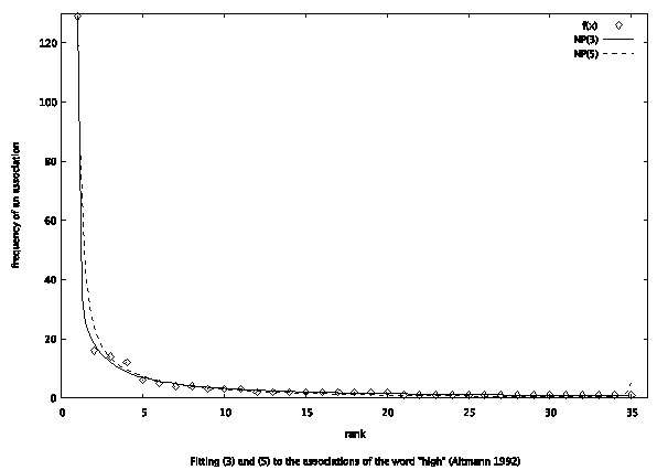
Altmann (1992) used the associations of the word “high” (4th grade, male) from Palermo, Jenkins (1964) and obtained the result presented in Table 1 and Fig. 1.
Both results are excellent.
4. Authors: U. Strauss, G. Altmann, J. Eom
5. References:
Altmann, G. (1992). Two models for word association data. Glottometrika 13, 105-120.
Altmann, G., Bagheri, D., Goebl, H., Köhler, R., Prün, C. (2002). Einführung in die quantitative Lexikologie. Götingen: Peust & Gutschmidt.
Dolinskij, V.A. (1994). Moscow Student´s word associations. In: 2nd International Conference on Quantitative Linguistics, September 20-24, 1994, Moscow: 66-68. Moscow: Lomonosov Moscow State University.
Dolinskij, V.A. (1988). Raspredelenie reakcij v ekseprimentach po verbal´nym associacijam. Acta et Commentationes Universitatis Tartuensis 827, 80-101.
Haight, F.A. (1966). Some statistical problems in connection with word association data. J. of Mathematical Psychology 3, 217-233.
Haight, F.A., Jones, R.B. (1974). A probabilistic treatment of qualitative data with special reference to word association tests. J. of Mathematical Psychology 11, 237-244.
Horvath, W.J. (1963). A stochastic model for word association tests. Psychological Review 70, 361-364.
Hřebíček, L. (1995). Text levels. Language constructs, constituents and Menzerath-Altmann law. Trier: WVT.
Hřebíček, L. (1996). Word associations and text. Glottometrika 15, 12-17.
Hřebíček, L. (1997). Lectures on text theory. Prague: Oriental Institute.
Lánský, P., Radil-Weiss, T. (1980). A generalization of the Yule-Simon model, with special reference to word association tests and neural cell assembly formation. J. of Mathematical Psychology 21, 53-65.
Palermo, D.S., Jenkins, J.J. (1964): Word association norms. Grade School through College. Minneapolis: University of Minnesota Press.
Wimmer, G., Altmann, G. (1999). Thesaurus of univariate discrete probability distributions. Essen: Stamm.

