Gap formation

1. Problem and history

The distance (gap) between two identical entities in text can be measured in two ways: (i) in terms of the number of other intervening entities and (ii) as the number of steps from the previous occurrence of the entity to the next one. In the sequence

1 0 0 0 1

method (i) results in a gap of length 3, method (ii) yields 4. However, some entities cannot occur in direct neighbourhood, e.g. the same preposition.

The entities can be of any kind: word classes, lengths, structural types, clause types, phonemes, individual words occurring x-times, types of verse, etc.

The investigation was initiated by G.K. Zipf, who found different aspects of distances, or intervals, or gaps, between identical entities in text (Zipf 1935, 1937a,b, 1945, 1946, 1949). The first models were set up by Spang-Hanssen (1956), Yngve (1956) and Uhlířová (1967). Herdan (1966: 127-130) and Králík (1977) considered the gap as the time between two consecutive Poisson events and obtained the exponential distribution. Brainerd (1976) considered the sequence of entities as a two-state Markov chain and derived models of different order. Strauß, Sappok, Diller, and Altmann (1984) considered identical entities as an urn and derived the negative binomial distribution using the Poisson pure birth model. Zörnig (1984a,b) derived the model for the random distribution of distances. Hrebicek (2000), leaning against his general text theory, found that even distances abide by Menzerath´s law.

2. Hypothesis

According to a generalized Skinner hypothesis the probability of a small distance (gap) between identical entities in text is greater than the probability of greater distances. The hypothesis is based on the reinforcement of a stimulus which dies away.

Corollary: If Skinner´s hypothesis does not hold, then the gaps are distributed randomly and follow the Zörnig model (see below).

3. Derivations

3.1. The geometric model

Spang-Hanssen (1956), Yngve (1956) and Uhlířová (1967) assumed that if the probability of an entity A is p and that of non-A 1 - p = q, then the probability of a distance of size x is given simply by the geometric distribution

(1) $P_x = pq^x$, x = 0,1,2,…

which is adequate in many cases.

3.2. Markov chain model

Since the geometric distribution represents merely a Markov chain of zeroth order, not taking sequential dependencies into account, Brainerd (1976) considered higher chain orders and operated with transitions between elements A (= 1) and non-A (= 0). For the first order chain, he obtained the probability of no distance (x = 0) from the transition 11 as P(1|1). For all other distances, we consider 100…01, which means that there is a transition from 1 to 0 in the first step, then x-1 transitions between zeroes, P(0|0), and finally the transition from 0 to 1, yielding $P(0|1)P(1|0)P(0|0)^{x-1}$. In a similar way one can obtain dependencies of higher order. For the first three orders he obtained the following distributions:

(2) $P_x = \begin{cases} P(1|1), & \quad x=0 \\ P(0|1)P(1|0)P(0|0)^{x-1},& \quad x=1,2,...\end{cases}$

(3)$P_x= \begin{cases} P(1|1), & \quad x=0\\P(0|1)P(1|0),& \quad x=1\\P(0|1)P(0|10)P(1|00)P(0|00)^{x-2}, & \quad x=2,3,...\end{cases}$

(4)$P_x= \begin{cases} P(1|1), & \quad x=0\\P(01|1),& \quad x=1\\P(00|1)P(1|100), & \quad x=2\\P(00|1)P(0|100)P(1|000)P(0|000)^{x-3}, & \quad x=3,4,...\end{cases}$

One sees that the higher the order of the chain, the more extensive is the modification of the simple geometric distribution. For example (4) can be simply written as

$P_x = \begin{cases}\alpha, & \quad x=0\\\beta, & \quad x=1\\\gamma, & \quad x=2\\ (1-\alpha-\beta-\gamma)pq^{x-3}, & \quad x=3,4,...\end{cases}$

The parameters could express some properties of the given entity but there are no further exmanations in this direction. There are two problems with this approach: (a) Markov chains do not consider forward dependencies which are usual in text, (b) stepwise modification would capture any empirical distribution but at costs of explanatory power. A simple description of these chains can be found in Altmann (1988a) and a survey of modified distribution in Wimmer, Witkovský, Altmann (1999).

3.3. Urn model

The derivations in 3.1 and 3.2 do not take Skinner´s hypothesis into account, they are rather of local character. Strauß, Sappok, Diller and Altmann (1984) consider two occurrences of element A as an urn which exerts influence on acceptance or rejection of new non-A elements. Let the placement of non-A elements between two A elements be a Poisson pure birth process (see Appendix) in which new non-A elements can only be inserted but not taken away, yielding

(5)$P^'_0(t)=-\lambda_0P_0(t)$

$P^'_x(t)=-\lambda_xP_x(t)+\lambda_{x-1}P_{x-1}(t), \quad x=1,2,3,...$

If there is no trend, i.e. the “balls” fall in the urns randomly, then $\lambda_x= a$ (a constant) and the process results in the Poisson distribution. If however, the urns exert influence, the result may be different. If an urn repells new balls the more, the more balls are already in it, then one can write $\lambda_x= n-x$, insert it in (5), and obtain the binomial distribution.

However, Skinner´s hypothesis says that there is a tendency to produce more small distances and enlarge the long ones. This means that an urn attracts the more new balls the more are already in it. Substituting in $\lambda_x = k+x$ in (5), one obtains

(6)$P^'_0(t)=-kP_0(t),$

$P^'_x(t)=-(k+x)P_x(t)+(k-x-1)P_{x-1}(t), \quad x=1,2,3...$

Solving (6) in the usual way and setting e-t = q, one obtains the negative binomial distribution

(7)$P_x = \left( \frac{k+x-1}{x}\right)p^kq^x, \quad x=0,1,2,...; \quad k>0; \quad 0<p<1; \quad q=1-p$

Example: Distances between equal rhythmic structures in hexameter

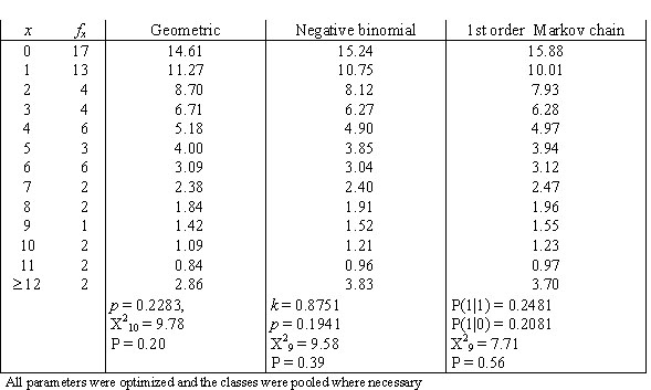
Strauß et al. (1984) examined the occurrence of verses with the structure DSSS (D – dactylus, S – spondeus) in 300 lines of Bridges´ “Poems in Classical prosody. Epistle II: To a Socialist in London” and recorded the distances between them. They obtained the results in the first and the second columns of Table 1. The geometric d., the negative binomial d. and the Markov chain of first order were fitted to these data.

Table 1 Fitting of distance models to the data of Strauß et al. (1984)

As it can be seen, the first order Markov chain yields the best fit for this type of data.

3.4. The Menzerathian model

Starting from a different philosophy of texts, Hřebíček (2000) assumes that not only hierarchical relations but also sequential ones abide by the simplest form of Menzerath´s law (for derivation see Hierarchic relations) yielding

(8) $y_x=ax^{-b}$,

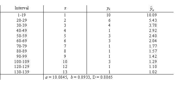
where $y_x$ is the frequency of the distance x between identical units. It can be considered either as a usual function (without norming), or as a probability function representing the zeta distribution (a being the norming constant and b > 1). Testing with good results has been performed for words of high frequency in Czech and Turkish (Hřebíček 2000). Hřebíček used method (ii) for measuring distances and still another method consisting of counting the intervening sentences.

Example: Distances between the personal name “Nihat” in a Turkish text

Hřebíček (2000: 32-34) pooled the distances in intervals and obtained the results presented in Table 2.

Table 2 Distances between the name “Nihat” in a Turkish text (Hřebíček 2000)

The fitting is satisfactory.

3.5. Zörnig´s model of random distribution of distances between any number of identical entities (Zörnig 1984a,b).

In the above models the entities of the text were always divided dichotomically to elements A and non-A. One can also add all distances of the same size or examine the distances for each element separately. If the distances between identical entities are random, then they follow the distribution

(9)$P_x = \frac {(n-x-1)!}{n!(n-m)}\sum_{i=1}^m k_i(k_i-1)(n-k_i)_{(x)}$,

or, if we are interested in fequencies, we have, with N = n-m,

(10)$NP_x = \frac{(n-x-1)!}{n!}\sum_{i=1}^m k_i (k_i-1)(n-k_i)_{(x)}$

where

n = number of elements in the sequence

m = number of different element types

$k_i$ = frequency of occurrence of elements of type i (i = 1,2,...,m)

$r_{(x)} = r(r-1)(r-2)...(r-x+1)$

Example: Distances in an artificial case

Let us consider the following sequence:

A B A C D B C A D D B

Here

n = 11

m = 4 (A,B,C,D)

$k_1 = k_A = 3$

$k_2 = k_B = 3$

$k_3 = k_C = 2$

$k_4 = k_D = 3$

We find here following distances:

Between the A´s 1 and 4

Between the B´s 3 and 4

Between the C´s 2

Between the D´s 3 and 0

Using (2) we compute the theoretical frequency of distance 2:

$NP_2=\frac{(11-2-1)!}{11!}(3(3-1)(11-3)(11-2)+3(3-1)(11-3)(11-2)+2(2-1)(11-2)(11-1)+3(3-1)(11-3)(11-2)=1.3553.$

In the same way one can compute the other distances and compare them with the real ones.

4. Authors: U. Strauss, G. Altmann, L. Hřebíček

5. References

Altmann, G. (1988a). Wiederholungen in Texten. Bochum, Brockmeyer.

Brainerd, B. (1976). On the Markov nature of text. Linguistics 176, 5-30.

Chen, Y.-S. (1988). An exponential recurrence distribution in the Simon-Yule model of text. Cybernetics and Systems: An International Journal 19, 521-545.

Chen, Y.-S., Chong, P.P., Kim, J.-S. (1992). A self-adaptive statistical language model for speech recognition. Cybernetica 35(2), 103-127.

Herdan, G. (1966). The advanced theory of language as choice and chance. Berlin, Springer (p. 127-130).

Hřebíček, L. (2000). Variation in sequences. Prague: Oriental Institute

Králík, J. (1977). An application of exponential distribution law in quantitative linguistics. Prague Studies in Mathematical Linguistics 5, 223-235.

Prün, C. (1997). A text linguistic hypothesis of G.K. Zipf. J. of Quantitative Linguistics 4, 244-251.

Spang-Hanssen, H. (1956). The study of gaps between repetitions. In: Halle, M. (Ed.), For Roman Jakobson: 497-502. The Hague: Mouton.

Strauß, U., Sappok, Ch., Diller, H.J., Altmann, G. (1984). Zur Theorie der Klumpung von Textentitäten. Glottometrika 7, 73-100.

Uhlířová, L. (1967). Statistics of word order of direct object in Czech. Prague Studies in Mathematical Linguistics 2, 37-49.

Wimmer, G., Witkovský, V., Altmann, G. (1999). Modification of probability distributions applied to word length research. J. of Quantitative Linguistics 6, 257-268.

Yngve, V. (1956). Gap analysis and syntax. IRE Transactions PGIT-2, 106-112.

Zipf, G.K. (1935). The psycho-biology of language: an introduction to dynamic phlology. Boston: Houghton Mifflin.

Zipf, G.K. (1937a). Observations on the possible effect of mental age upon the frequency-distribution of words from the viewpoint of dynamic philology. Journal of Psychology 4, 239-244.

Zipf, G.K. (1937b). Statistical methods in dynamic philology (Reply to M. Joos). Language 132, 60-70.

Zipf, G.K. (1945). The repetition of words, time-perspective and semantic balance. The J. of General Psychology 32, 127-148.

Zipf, G.K. (1946). The psychology of language. In: Hariman, P.L. (ed.), Encyclopedia of Psychology: 332-341. New York: Philosophical Library.

Zipf, G.K. (1949). Human behavior and the principle of least effort. Cambridge/Mass.: Addison-Wesley.

Zörnig, P. (1984a). The distribution of the distance between like elements in a sequence I. Glottometrika 6, 1-15.

Zörnig, P. (1984b). The distribution of the distance between like elements in a sequence II. Glottometrika 7, 1-14.

Zörnig, P. (1987). A theory of distances between like elements in a sequence. Glottometrika 8, 1-22.